INTERACTIVE_NETWORK#

This module is a part of metaFun pipeline, providing an interactive web interface for microbial co-occurrence network analysis and visualization.
Overview#
The INTERACTIVE_NETWORK module offers a dynamic, web-based platform for constructing, analyzing, and visualizing microbial co-occurrence networks. It allows researchers to build correlation-based networks using FastSpar (compositional data) or FlashWeave (conditional independence), compare network properties across sample groups, identify influential taxa through centrality analysis, and assess network robustness. The module leverages phyloseq objects to enable advanced network analyses and customizable visualizations without requiring programming knowledge.
Key Capabilities:
Network inference using FastSpar (SparCC) or FlashWeave (conditional independence)
Group-wise network comparison with topology metrics
Influential node detection via Zi-Pi classification and IVI scores
Network robustness analysis using brainGraph attack simulations
Interactive visualization with real-time threshold adjustment
This module enables group-wise network comparison, allowing users to construct separate networks for different conditions (e.g., healthy vs. disease) and compare their structural properties.
Module Execution#
This module takes the phyloseq RDS output from the WMS_TAXONOMY module as input.
Pipeline Integration:
WMS_TAXONOMY → phyloseq.rds → INTERACTIVE_NETWORK
# Basic usage with phyloseq RDS file
(metafun) metafun -module INTERACTIVE_NETWORK -i results/metagenome/WMS_TAXONOMY/phyloseq/phyloseq_object.RDS

# Specify custom port for the web interface
(metafun) metafun -module INTERACTIVE_NETWORK -i results/metagenome/WMS_TAXONOMY/phyloseq/phyloseq_object.RDS -p 8080

# Use phyloseq from Sylph profiling
(metafun) metafun -module INTERACTIVE_NETWORK -i results/metagenome/WMS_TAXONOMY/phyloseq/phyloseq_object_sylph.RDS
Module Operation Sequence#
This module performs the following steps:
Step 1: Load Data
Upload phyloseq RDS file from WMS_TAXONOMY output
Select grouping variable from sample metadata
Review data summary in Data Overview tab
Step 2: Configure Filtering
Set taxonomic aggregation level (Species, Genus, Family, etc.)
Adjust prevalence threshold (default: 10%)
Set minimum relative abundance (default: 0.1%)
Step 3: Select Network Method
FastSpar: For standard compositional correlation with bootstrap p-values
FlashWeave: For conditional independence-based network inference
Step 4: Run Analysis
Click “Run Network Analysis” button
Wait for computation (progress shown in console)
Step 5: Explore Results
Network Analysis tab: Compare topology metrics across groups
Influential Nodes tab: Identify hub taxa via Zi-Pi plot and IVI
Network Robustness tab: Run stability tests (optional)
Network Visualization tab: Interactive network exploration
Step 6: Export Results
Download tables (CSV) and networks (GraphML) for external analysis
Parameters#
This module has no command-line parameters. All configuration is performed through the interactive interface.
The phyloseq RDS object is the sole required input.
Inputs and Outputs#
Inputs#
Phyloseq RDS file from WMS_TAXONOMY module
Phyloseq object must contain: OTU table, taxonomy table, and sample metadata
Outputs#
Interactive network visualizations
Network comparison statistics
Node centrality tables
Influential taxa rankings
Robustness analysis results
Exportable figures and data tables
Output directory structure#
The generated files are saved in the application’s output directory:
${launchDir}/results/interactive_network/
├── exported_figures/                      # Exported visualizations
│   ├── network_[group]_[timestamp].pdf         # Network diagrams
│   ├── comparison_metrics_[timestamp].pdf      # Group comparison plots
│   ├── influential_nodes_[timestamp].pdf       # Centrality analysis plots
│   └── robustness_analysis_[timestamp].pdf     # Robustness curves
├── network_results/                       # Network analysis outputs
│   ├── edge_list_[group]_[timestamp].csv       # Edge lists per group
│   ├── node_metrics_[group]_[timestamp].csv    # Node centrality metrics
│   ├── comparison_table_[timestamp].csv        # Group comparison statistics
│   └── correlation_matrix_[group].csv          # Raw correlation matrices
└── analysis_logs/                         # Processing logs
    └── network_analysis_[timestamp].log        # Analysis parameters and results
Interface Components#
The web interface is divided into multiple tabs, each providing specialized tools for different types of network analysis.
1. Main Interface Overview#
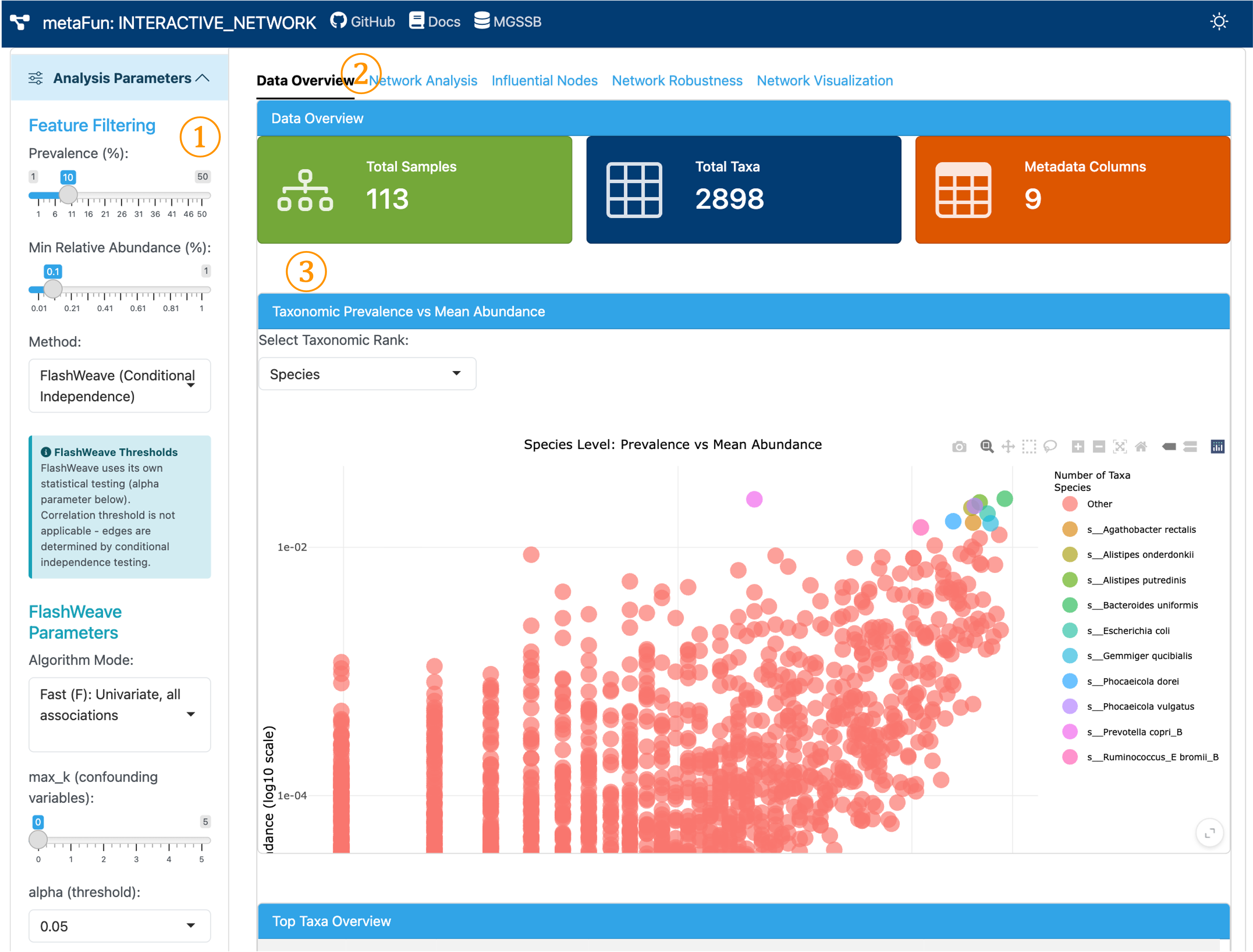
① Sidebar (Analysis Parameter Settings): Configure prevalence and abundance filtering conditions, select co-occurrence network method, and set parameters for network generation.
② Navigation Tabs: Access different analysis modules within the network application:
Data Overview: Summary of loaded phyloseq data and filtering preview
Network Analysis: Network topology metrics and edge distribution comparison
Influential Nodes: Zi-Pi classification and node centrality analysis
Network Robustness: Stability testing through node removal simulations
Network Visualization: Interactive network graph with customizable display
③ Main Content Area: Displays tables, plots, and analysis results corresponding to each selected tab.
2. Sidebar Panel (Master Controller)#
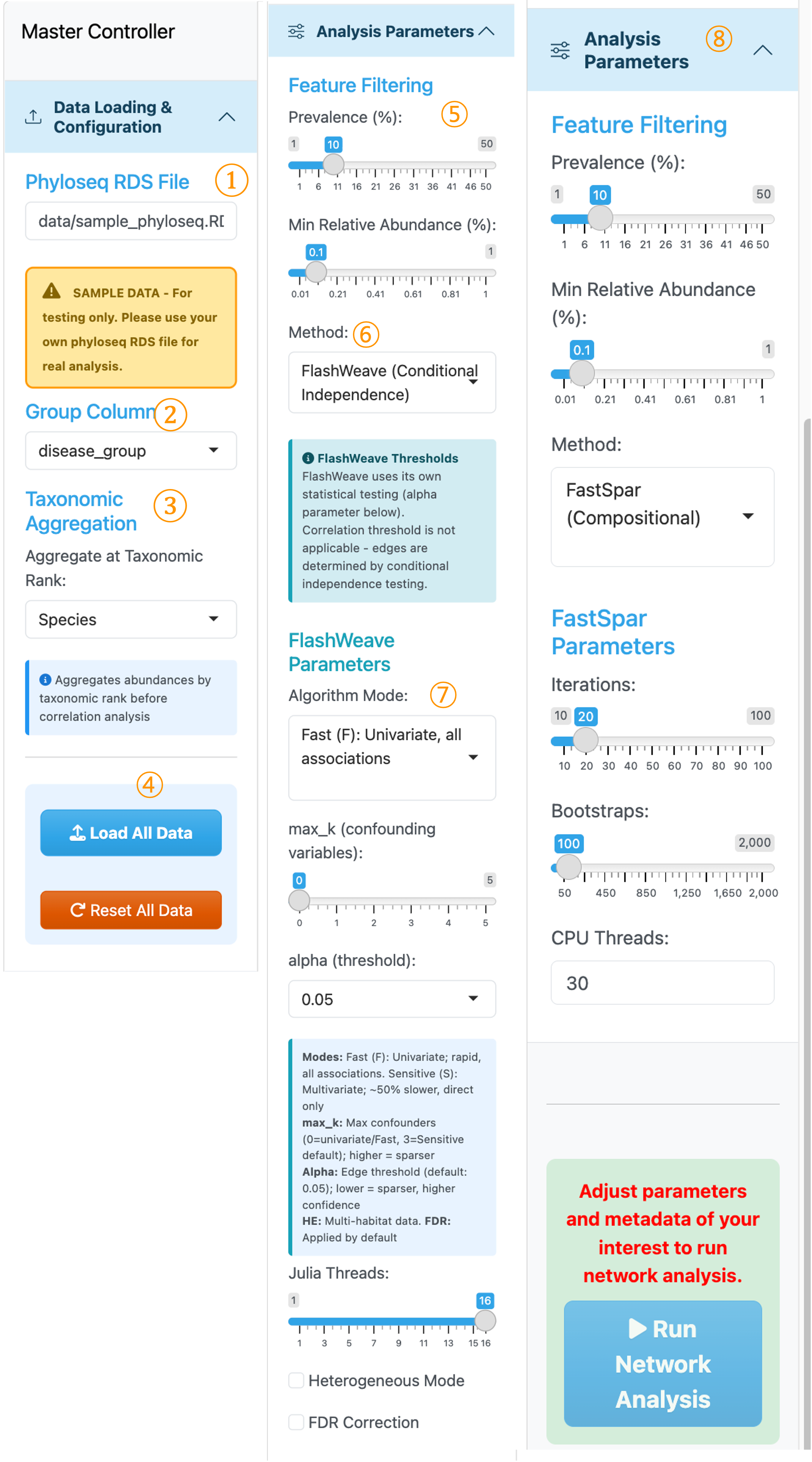
① Phyloseq RDS File: A sample phyloseq object is pre-loaded for testing. We recommend using your own data from the WMS_TAXONOMY module output.
② Group Column: Select metadata variable for group-wise network comparison. Separate networks will be generated for each category. Currently supports categorical variables only.
③ Taxonomic Aggregation: Aggregate taxa with identical taxonomic information at a specific rank for visualization and analysis.
④ Load All Data / Reset All Data: Buttons to load the phyloseq data into the application or reset to default settings.
⑤ Prevalence & Relative Abundance Filtering: Adjust thresholds to filter out rare taxa and prevent excessive zero counts in the abundance matrix, which can affect correlation estimation.
⑥ Method Selection: Choose between FlashWeave (Conditional Independence) or FastSpar (Compositional) for network inference.
⑦ FlashWeave Parameters: Parameter settings for FlashWeave analysis. Configure algorithm mode, alpha threshold, and other options according to your research objectives before running network generation.
⑧ FastSpar Parameters: Parameter settings displayed when FastSpar is selected. Set appropriate thresholds for iterations, bootstraps, and significance before proceeding with network construction.
Note
FlashWeave vs FastSpar:
FlashWeave: Uses conditional independence testing to detect direct associations while filtering out indirect effects. Best for identifying true ecological interactions.
FastSpar: C++ implementation of SparCC, specifically designed for compositional data. Accounts for the compositional nature of microbiome data where relative abundances sum to a constant, avoiding spurious correlations that arise from standard correlation methods. Provides bootstrap p-values for significance testing.
3. Network Analysis Tab#
This tab displays network characteristics and allows comparison of positive/negative edge distributions across taxonomic groups.
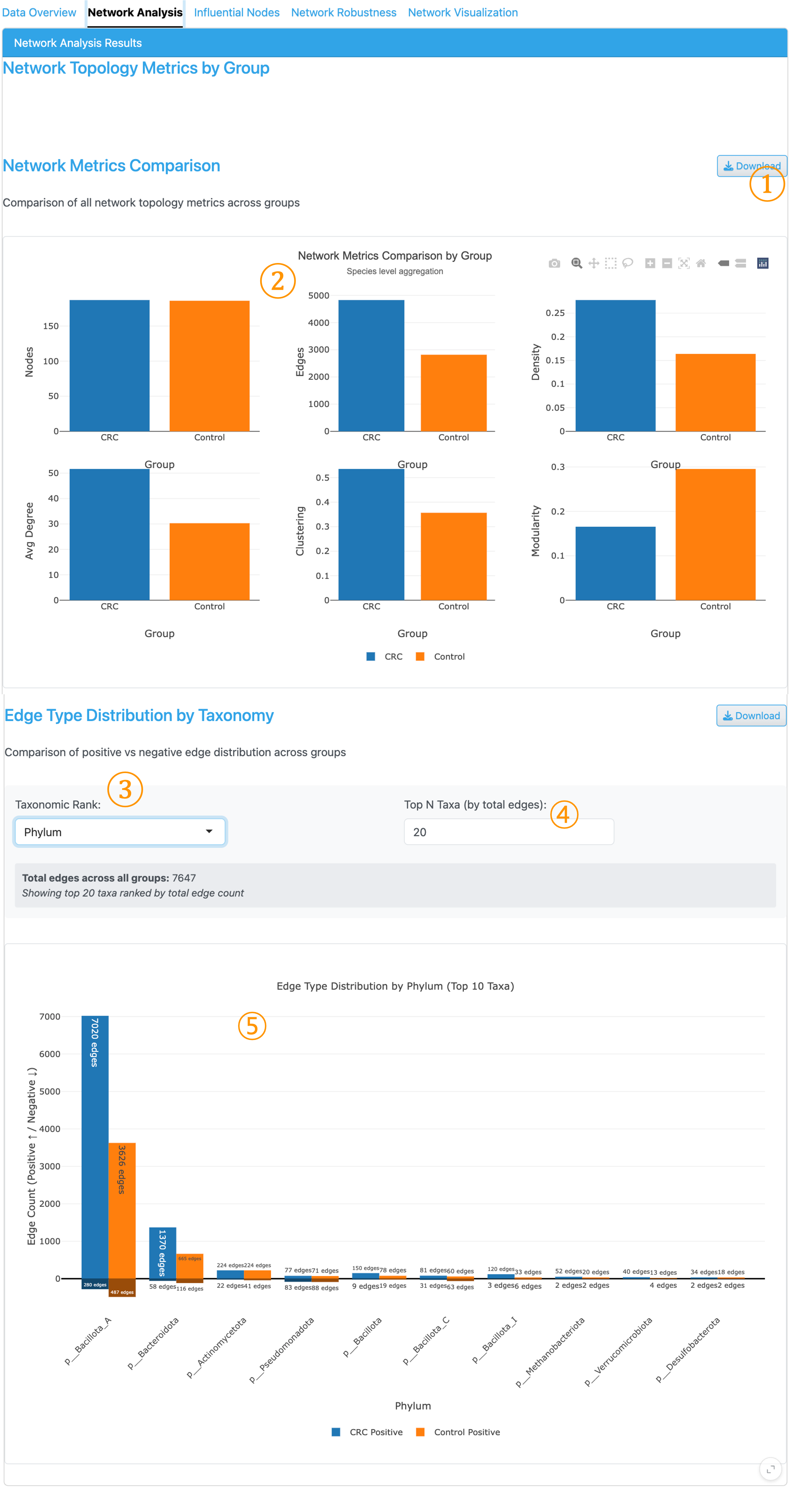
① Download Button: Export the visualization with customizable settings (format, size, resolution) for publication-ready figures.
② Network Metrics Comparison: Faceted bar chart comparing fundamental network properties across groups, enabling quick assessment of structural differences between condition-specific networks.
③ Taxonomic Rank Selector: Nodes are based on the taxonomic rank selected in the sidebar. This selector determines the rank level for aggregating edge counts to calculate proportions.
④ Top N Taxa: Number of top taxa to display in the edge distribution plot.
⑤ Edge Type Distribution Plot: Stacked bar chart showing the ratio of positive and negative edges by taxonomic group, allowing quick comparison of co-occurrence patterns between groups.
Network Metrics Explained:
Nodes: Number of taxa with at least one significant correlation. Higher node counts indicate more taxa participating in the network.
Edges: Number of significant pairwise correlations. Represents the total connections in the network.
Density: Proportion of possible edges that actually exist (edges / maximum possible edges). Values range from 0 to 1, with higher values indicating more interconnected networks.
Avg Degree: Mean number of connections per node. Higher average degree suggests taxa are more interconnected on average.
Clustering (Transitivity): Proportion of closed triangles among connected triplets. Measures the tendency of nodes to cluster together, indicating modular structure.
Modularity: Strength of community structure ranging from 0 to 1. Higher values indicate distinct modules or communities within the network, suggesting functional or ecological groupings.
4. Download Plot Dialog#
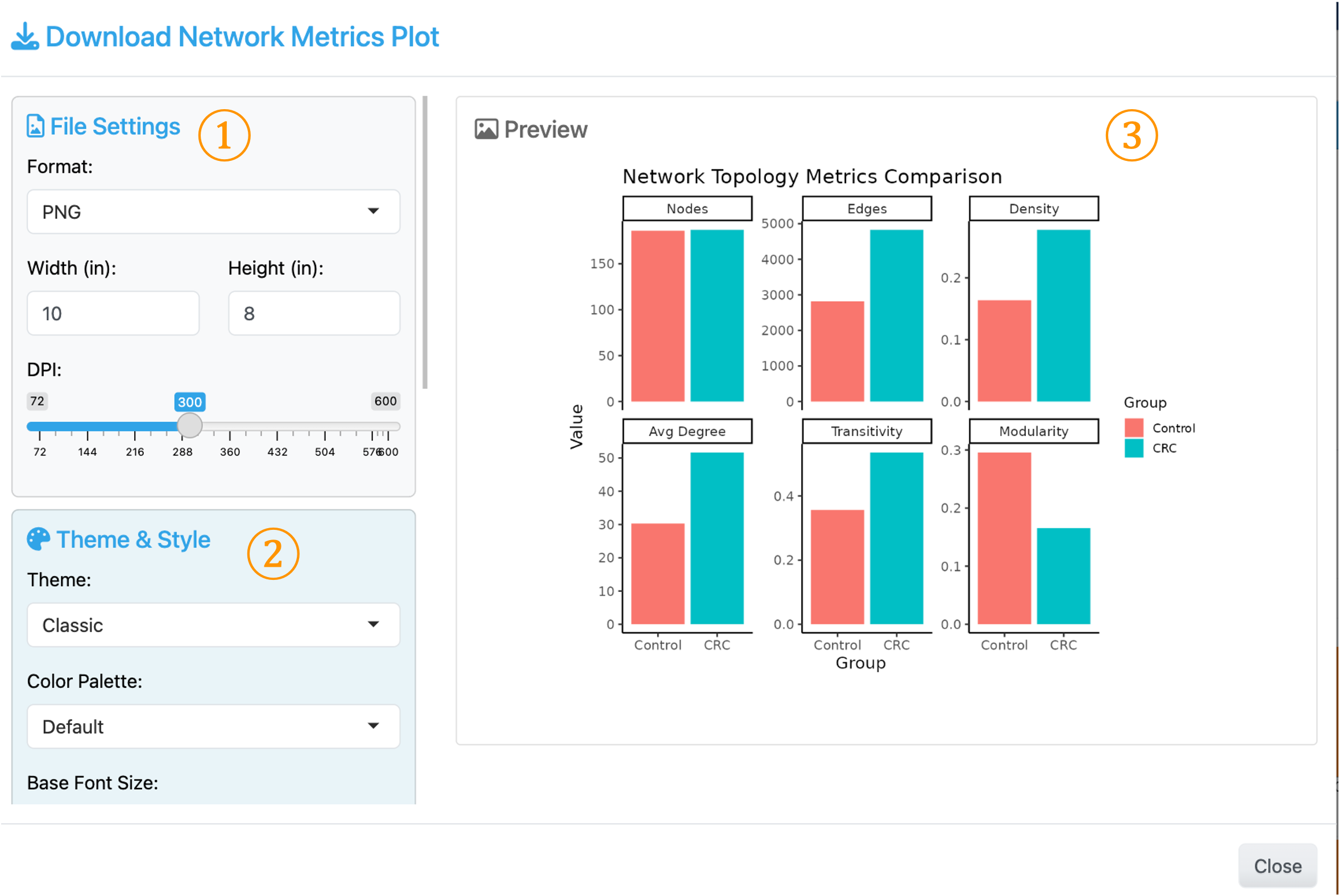
① File Settings: Format (PNG/PDF/SVG), Width, Height (inches), DPI (72-600)
② Theme & Style: Theme selection (Classic, Minimal, etc.), Color Palette, Base Font Size
③ Preview: Real-time preview of the plot with current settings
5. Influential Nodes Tab (Zi-Pi Analysis)#
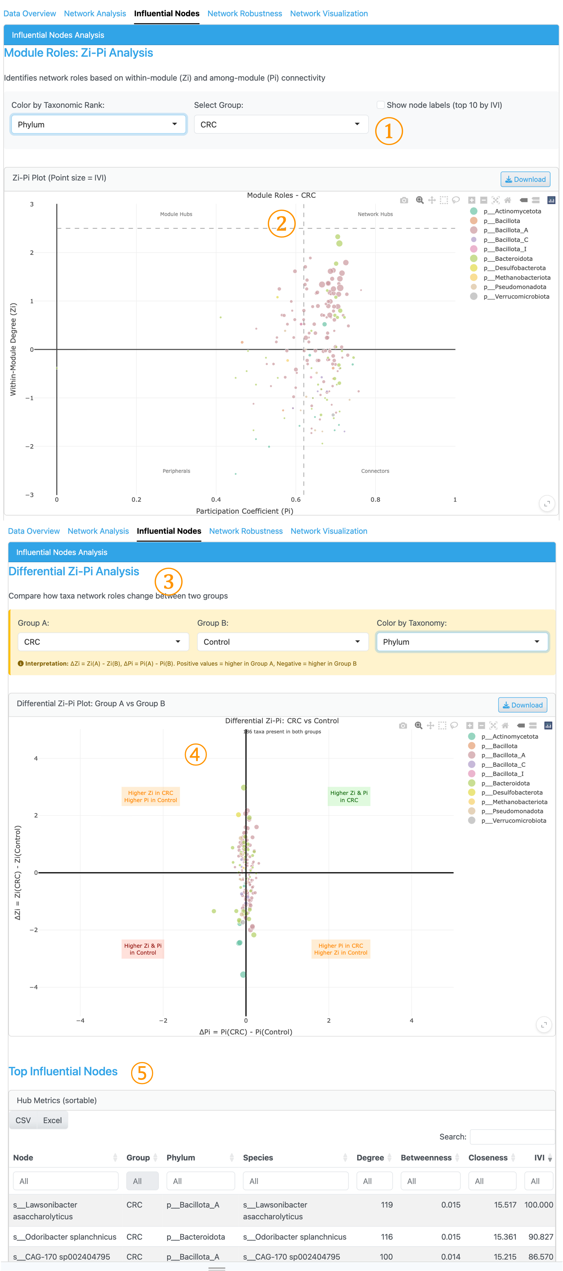
① Group Selector: Select which metadata group’s network to visualize for node influence analysis. Nodes are displayed based on the taxonomic rank selected in the sidebar controller. Node coloring by higher taxonomic rank is available.
② Zi-Pi Plot: Scatter plot visualizing node roles with Within-module degree (Zi) on y-axis and Participation coefficient (Pi) on x-axis. Hover over points to see detailed Zi, Pi, and IVI values. Point size represents the Integrated Value of Influence (IVI), a comprehensive metric combining multiple centrality measures (Salavaty et al., 2020). Dashed lines at Zi=2.5 and Pi=0.62 define four role quadrants for node classification.
③ Differential Zi-Pi Analysis: Compare node centrality metrics between two groups to identify taxa with significantly different network roles. Select the two groups to compare.
④ Differential Zi-Pi Plot: Shows ΔZi vs ΔPi between the selected groups, highlighting nodes with substantial differences in network position across conditions.
⑤ Top Influential Nodes Table: Numeric summary of node influence metrics including IVI, degree, betweenness, and closeness centrality for detailed quantitative assessment.
Zi-Pi Role Classification:
Network Hubs (Zi > 2.5, Pi > 0.62): Keystone taxa connecting multiple modules
Module Hubs (Zi > 2.5, Pi ≤ 0.62): Central within their module
Connectors (Zi ≤ 2.5, Pi > 0.62): Bridge taxa linking modules
Peripherals (Zi ≤ 2.5, Pi ≤ 0.62): Specialists with limited influence
6. Group-Specific Taxa Analysis (Influential Nodes Tab)#
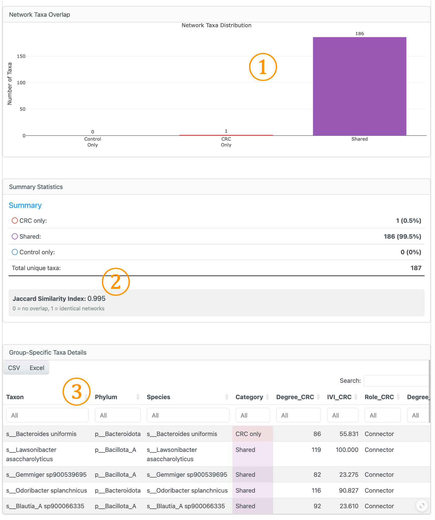
This section facilitates identification of nodes unique to specific groups through visualization and tabular summary.
① Network Taxa Distribution: Bar chart and summary enabling easy identification of nodes present only in specific groups versus shared nodes.
② Network Similarity (Jaccard Index): Calculates the similarity between two group networks based on shared nodes. Values range from 0 (no overlap) to 1 (identical node composition).
③ Group-Specific Taxa Details: Sortable table displaying node information with group membership, based on the taxonomic rank selected in the master controller.
7. Network Robustness Tab#
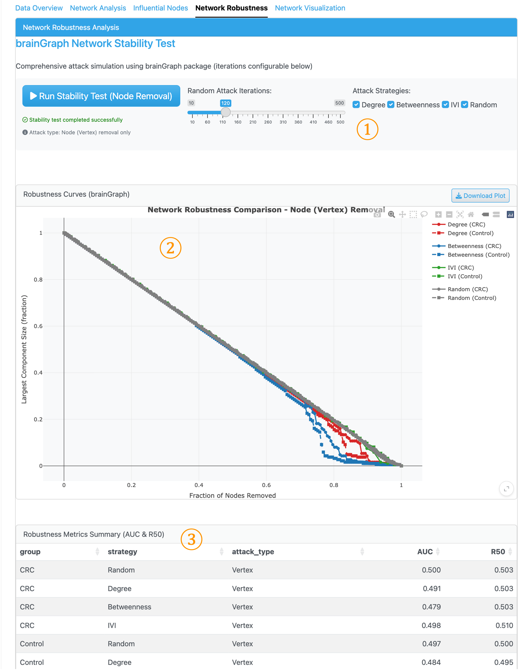
This tab uses brainGraph to assess network stability by simulating node removal and measuring the resulting network fragmentation. This analysis reveals how resilient each network is to perturbation.
① Stability Test Controls: Configure attack strategies for node removal simulation. Options include targeted attacks (removing nodes by Degree, Betweenness, or IVI) and random removal.
② Robustness Curves: Line plot showing how the Largest Component Size decreases as nodes are progressively removed. Steeper curves indicate more vulnerable networks.
③ Robustness Metrics Summary: Quantitative assessment with AUC and R50 values. Lower values indicate faster network collapse, suggesting the network is more dependent on key hub taxa for maintaining connectivity.
Interpreting Network Robustness
Network robustness analysis helps identify how ecological communities respond to species loss. Networks that collapse quickly under targeted attacks (low AUC, low R50) are more vulnerable to keystone species removal. The gap between random and targeted attack curves indicates hub dependency—larger gaps suggest the network relies heavily on a few influential taxa for structural integrity (Dunne et al., 2002; Coyte et al., 2015).
8. Network Visualization Tab#

This tab provides interactive network visualization with customizable display settings, along with detailed node and module information.
① Visualization Settings: Configure view mode (side-by-side comparison or single group), layout algorithm, node coloring (by taxonomy, degree, or module), node sizing (by IVI, degree, or betweenness), edge opacity, and correlation strength filter.
② Network Graph: Interactive plotly visualization. Hover over nodes to see taxon details. Green edges indicate positive correlations; red edges indicate negative correlations.
③ Node Properties Table: Detailed centrality metrics for each node including degree, betweenness, closeness, and eigenvector centrality.
④ Module Assignment Table: Community detection results showing module membership, allowing exploration of functional or ecological groupings within the network.
Download Options:
Download Network Plot: Export visualization as image
Download GraphML: Export network for Cytoscape/Gephi
Network Methods#
FastSpar (Default)#
FastSpar is an efficient implementation of SparCC for compositional data:
Purpose: Estimates correlations from compositional (relative abundance) data
Approach: Iterative algorithm to handle compositional bias
Parameters:
Iterations: Number of iterations for correlation estimation (10-100)
Bootstraps: Number of bootstrap replicates for p-values (50-2000)
Threads: CPU threads for parallel processing
FastSpar advantages
FastSpar is recommended for microbiome data because it:
Handles compositional bias inherent in relative abundance data
Provides bootstrap-based p-values for statistical filtering
Allows post-hoc threshold adjustment without re-running
FlashWeave#
FlashWeave uses conditional independence testing for network inference:
Purpose: Identifies direct associations, filtering indirect effects
Approach: Tests for conditional independence given confounders
Parameters:
Algorithm mode: Fast (univariate) or Sensitive (multivariate)
max_k: Maximum confounding variables to consider
alpha: Statistical threshold for edge inclusion
FDR: False discovery rate correction
FlashWeave advantages
FlashWeave is useful when:
Distinguishing direct from indirect associations is important
Sample size is sufficient for conditional testing
Sparser, more biologically meaningful networks are desired
Usage Notes#
Choosing Network Inference Method:
FastSpar: Best for standard compositional analysis with bootstrap p-values. Key parameters: Iterations (20-100), Bootstraps (100-2000)
FlashWeave: Best for large datasets, direct associations, FDR control. Key parameters: alpha (0.01-0.1), max_k (0-5), Sensitive/Fast mode
Performance Recommendations:
For >500 taxa: Use FlashWeave Fast mode or increase FastSpar threads
For visualization: Filter to top 100-200 taxa for clarity
For publication: Use ≥100 bootstrap iterations (FastSpar) or Sensitive mode (FlashWeave)
Example Workflows#
Workflow 1: Basic Group Comparison
Load phyloseq from WMS_TAXONOMY output
Select grouping variable (e.g., “disease_group”)
Set Species-level aggregation
Choose FlashWeave with default parameters
Click “Run Network Analysis”
Compare network metrics in Network Analysis tab
Identify differential hubs using Zi-Pi analysis
Workflow 2: Keystone Taxa Identification
Complete network analysis
Navigate to Influential Nodes tab
Examine Zi-Pi plot for Network Hubs and Module Hubs
Use Differential Zi-Pi to compare hub status across groups
Check Group-Specific Taxa for unique network members
Download hub metrics table for downstream analysis
Workflow 3: Network Stability Assessment
Complete network analysis
Go to Network Robustness tab
Set iterations to 100+
Select all attack strategies (Degree, Betweenness, IVI, Random)
Click “Run Stability Test”
Compare AUC values between groups
Identify which group has more hub-dependent structure
Key Programs#
Network Inference#
FastSpar: C++ implementation of SparCC for compositional correlation (Friedman & Alm, 2012)
FlashWeave: Julia-based network inference using conditional independence (Tackmann et al., 2019)
Network Analysis#
igraph: R package for network analysis and visualization
brainGraph: R package for network robustness simulations
influential: R package for IVI calculation (Salavaty et al., 2020)
Louvain: Community detection algorithm for module identification
References:
Friedman, J., & Alm, E. J. (2012). Inferring correlation networks from genomic survey data. PLoS Computational Biology, 8(9), e1002687.
Tackmann, J., et al. (2019). Rapid inference of direct interactions in large-scale ecological networks. Cell Systems, 9(3), 286-296.
Salavaty, A., et al. (2020). Integrated Value of Influence: An integrative method for the identification of the most influential nodes. Patterns, 1(5), 100052.
Guimerà, R., & Amaral, L. A. N. (2005). Functional cartography of metabolic networks. Nature, 433(7028), 895-900.
Coyte, K. Z., Schluter, J., & Foster, K. R. (2015). The ecology of the microbiome: Networks, competition, and stability. Science, 350(6261), 663-666.
Dunne, J. A., Williams, R. J., & Martinez, N. D. (2002). Network structure and biodiversity loss in food webs: robustness increases with connectance. Ecology Letters, 5(4), 558-567.